Eigenface-based facial recognition

Dimitri PISSARENKO

February 8, 2003

1 General

This document is based upon Turk and Pentland (1991b), Turk and Pentland (1991a) and Smith (2002).

2 How does it work?

The task of facial recogniton is discriminating input signals (image data) into several classes (persons). The input signals are highly noisy (e.g. the noise is caused by differing lighting conditions, pose etc.), yet the input images are not completely random and in spite of their differences there are patterns which occur in any input signal. Such patterns, which can be observed in all signals could be - in the domain of facial recognition - the presence of some objects (eyes, nose, mouth) in any face as well as relative distances between these objects. These characteristic features are called eigenfaces in the facial recognition domain (or principal components generally). They can be extracted out of original image data by means of a mathematical tool called Principal Component Analysis (PCA).
By means of PCA one can transform each original image of the training set into a corresponding eigenface. An important feature of PCA is that one can reconstruct reconstruct any original image from the training set by combining the eigenfaces. Remember that eigenfaces are nothing less than characteristic features of the faces. Therefore one could say that the original face image can be reconstructed from eigenfaces if one adds up all the eigenfaces (features) in the right proportion. Each eigenface represents only certain features of the face, which may or may not be present in the original image. If the feature is present in the original image to a higher degree, the share of the corresponding eigenface in the ”sum” of the eigenfaces should be greater. If, contrary, the particular feature is not (or almost not) present in the original image, then the corresponding eigenface should contribute a smaller (or not at all) part to the sum of eigenfaces. So, in order to reconstruct the original image from the eigenfaces, one has to build a kind of weighted sum of all eigenfaces. That is, the reconstructed original image is equal to a sum of all eigenfaces, with each eigenface having a certain weight. This weight specifies, to what degree the specific feature (eigenface) is present in the original image.
If one uses all the eigenfaces extracted from original images, one can reconstruct the original images from the eigenfaces exactly. But one can also use only a part of the eigenfaces. Then the reconstructed image is an approximation of the original image. However, one can ensure that losses due to omitting some of the eigenfaces can be minimized. This happens by choosing only the most important features (eigenfaces). Omission of eigenfaces is necessary due to scarcity of computational resources.
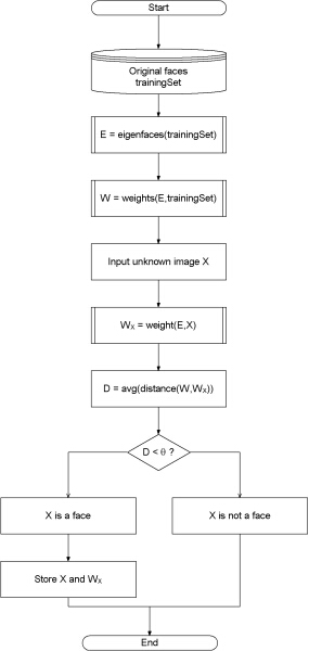
How does this relate to facial recognition? The clue is that it is possible not only to extract the face from eigenfaces given a set of weights, but also to go the opposite way. This opposite way would be to extract the weights from eigenfaces and the face to be recognized. These weights tell nothing less, as the amount by which the face in question differs from ”typical” faces represented by the eigenfaces. Therefore, using this weights one can determine two important things:

Determine, if the image in question is a face at all. In the case the weights of the image differ too much from the weights of face images (i.e. images, from which we know for sure that they are faces), the image probably is not a face.
Similar faces (images) possess similar features (eigenfaces) to similar degrees (weights). If one extracts weights from all the images available, the images could be grouped to clusters. That is, all images having similar weights are likely to be similar faces.

3 Overview over the algorithm

Figure 1:

High-level functioning principle of the eigenface-based facial recognition algorithm

The algorithm for the facial recognition using eigenfaces is basically described in figure 1. First, the original images of the training set are transformed into a set of eigenfaces E. Afterwards, the weights are calculated for each image of the training set and stored in the set W .
Upon observing an unknown image X, the weights are calculated for that particular image and stored in the vector W_X. Afterwards, W_X is compared with the weights of images, of which one knows for certain that they are faces (the weights of the training set W ). One way to do it would be to regard each weight vector as a point in space and calculate an average distance D between the weight vectors from W_X and the weight vector of the unknown image W_X (the Euclidean distance described in appendix A would be a measure for that). If this average distance exceeds some threshold value

, then the weight vector of the unknown image W_X lies too ”far apart” from the weights of the faces. In this case, the unknown X is considered to not a face. Otherwise (if X is actualy a face), its weight vector W_X is stored for later classification. The optimal threshold value

has to be determined empirically.

4 Eigenvectors and eigenvalues

An eigenvector of a matrix is a vector such that, if multiplied with the matrix, the result is always an integer multiple of that vector. This integer value is the corresponding eigenvalue of the eigenvector. This relationship can be described by the equation M × u = × u, where u is an eigenvector of the matrix M and is the corresponding eigenvalue.
Eigenvectors possess following properties:

They can be determined only for square matrices
There are n eigenvectors (and corresponding eigenvalues) in a n × n matrix.
All eigenvectors are perpendicular, i.e. at right angle with each other.

5 Calculation of eigenfaces with PCA

In this section, the original scheme for determination of the eigenfaces using PCA will be presented. The algorithm described in scope of this paper is a variation of the one outlined here. A detailed (and more theoretical) description of PCA can be found in (Pissarenko, 2002, pp. 70-72).

5.1 Step 1: Prepare the data

In this step, the faces constituting the training set (

_i) should be prepared for processing.

5.2 Step 2: Subtract the mean

The average matrix

has to be calculated, then subtracted from the original faces (

_i) and the result stored in the variable

_i:

	= _n	(1)
	_i = _i -	(2)

5.3 Step 3: Calculate the covariance matrix

In the next stept the covariance matrix C is calculated according to

-1- sum M T C = M PnP n n-1

(3)

5.4 Step 4: Calculate the eigenvectors and eigenvalues of the covariance matrix

In this step, the eigenvectors (eigenfaces) u_i and the corresponding eigenvalues

_i should be calculated. The eigenvectors (eigenfaces) must be normalised so that they are unit vectors, i.e. of length 1. The description of the exact algorithm for determination of eigenvectors and eigenvalues is omitted here, as it belongs to the standard arsenal of most math programming libraries.

5.5 Step 5: Select the principal components

From M eigenvectors (eigenfaces) u_i, only M' should be chosen, which have the highest eigenvalues. The higher the eigenvalue, the more characteristic features of a face does the particular eigenvector describe. Eigenfaces with low eigenvalues can be omitted, as they explain only a small part of characteristic features of the faces.
After M' eigenfaces u_i are determined, the ”training” phase of the algorithm is finished.

6 Improvement of the original algorithm

There is a problem with the algorithm described in section 5. The covariance matrix C in step 3 (see equation 3) has a dimensionality of N² × N², so one would have N² eigenfaces and eigenvalues. For a 256 × 256 image that means that one must compute a 65,536 × 65,536 matrix and calculate 65,536 eigenfaces. Computationally, this is not very efficient as most of those eigenfaces are not useful for our task.
So, the step 3 and 4 is replaced by the scheme proposed by Turk and Pentland (1991a):

C = -1-
M sum _n_n^T = AA^T (4)
L = A^TA L_n,m = _m^T_n (5)
u_l = sum v_lk_k l = 1,...,M (6)
where L is a M ×M matrix, v are M eigenvectors of L and u are eigenfaces. Note that the covariance matrix C is calculated using the formula C = AA^T, the original (inefficient) formula is given only for the sake of explanation of A. The advantage of this method is that one has to evaluate only M numbers and not N². Usually, M « N² as only a few principal components (eigenfaces) will be relevant. The amount of calculations to be performed is reduced from the number of prixels (N² × N²) to the number of images in the training set (M).
In the step 5, the associated eigenvalues allow one to rank the eigenfaces according to their usefulness. Usually, we will use only a subset of M eigenfaces, the M' eigenfaces with the largest eigenvalues.

7 Classifying the faces

The process of classification of a new (unknown) face _new to one of the classes (known faces) proceeds in two steps.
First, the new image is transformed into its eigenface components. The resulting weights form the weight vector _O_ _new^T

_k = u_k^T(_new - ) k = 1...M' (7)
_O_ _new^T = [ ]
w1 w2 ... wM' (8)
The Euclidean distance between two weight vectors d( _O_ _i, _O_ _j) provides a measure of similarity between the corresponding images i and j. If the Euclidean distance between _new and other faces exceeds - on average - some threshold value , one can assume that _new is no face at all. d( _O_ _i, _O_ _j) also allows one to construct ”clusters” of faces such that similar faces are assigned to one cluster.

A Euclidean Distance

Let¹ an arbitrary instance x be described by the feature vector
$x = [a1(x),a2(x),...,an(x)]$ (9)
where a_r(x) denotes the value of the rth attribute of instance x. Then the distance between two instances x_i and x_j is defined to be d(x_i,x_j):
$------------------ V~ sum n 2 d(xi,xj) = (ar(xi)- ar(xj)) r=1$ (10)

B Notation

I	Face image
N × N	Size of I
	Training set
_i	Face image i of the training set
_new	New (unknown) image
	Average face
M = \|\|	Number of eigenfaces
M'	Number of eigenfaces used for face recognition
C	Covariance matrix
X^T	Transposed X (if X is a matrix)
u	Eigenvector (eigenface)
	Eigenvalue
_i	Weight i
_i^T	Weight vector of the image i
	Threshold value

References

T. M. Mitchell. Machine Learning. McGraw-Hill International Editions, 1997.

D. Pissarenko. Neural networks for financial time series prediction: Overview over recent research. BSc thesis, 2002.

L. I. Smith. A tutorial on principal components analysis, February 2002. URL http://www.cs.otago.ac.nz/cosc453/student_tutorials/ principal_component%s.pdf. (URL accessed on November 27, 2002).

M. Turk and A. Pentland. Eigenfaces for recognition. Journal of Cognitive Neuroscience, 3(1), 1991a. URL http://www.cs.ucsb.edu/~mturk/Papers/ jcn.pdf. (URL accessed on November 27, 2002).

M. A. Turk and A. P. Pentland. Face recognition using eigenfaces. In Proc. of Computer Vision and Pattern Recognition, pages 586-591. IEEE, June 1991b. URL http://www.cs.wisc.edu/~dyer/cs540/handouts/mturk-CVPR91. pdf. (URL accessed on November 27, 2002).

	C = _n_n^T = AA^T	(4)
	L = A^TA L_n,m = _m^T_n	(5)
	u_l = v_lk_k l = 1,...,M	(6)